43 add data labels to scatter plot excel 2007

Clustered Column and Line Combination Chart - Peltier Tech If we plot XY scatter data on the chart, Excel treats the categories as if the first category is at X=1, the second at X=2, and so on. For the XY scatter data, we can consider the axis as a continuous numerical scale starting at the first category number minus 0.5 and ending at the last category number plus 0.5, or in our example, from 0.5 to 3.5. › dynamically-labelDynamically Label Excel Chart Series Lines • My Online ... Sep 26, 2017 · Great question. Pivot Charts won’t allow you to plot the dummy data for the label values in the chart as it wouldn’t be part of the source data, so the options are: 1. create a regular chart from your PivotTable and add the dummy data columns for the labels outside of the PivotTable. Not ideal if you’re using Slicers.

How to add secondary axis in Excel (2 easy ways) - ExcelDemy 2) Now go to Insert tab => click on the Recommended Charts command in the Charts window or click on the little arrow icon on the bottom right corner of the window. 3) This will open the Insert Chart dialog box. In the Insert Chart dialog box, choose the All Charts tab. Then choose the Combo option from the left menu.

Add data labels to scatter plot excel 2007

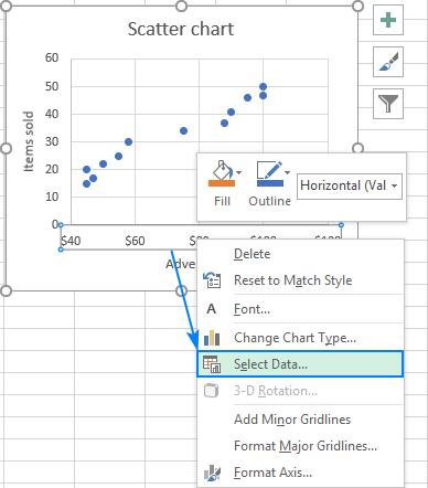
How to Create A Timeline Graph in Excel [Tutorial & Templates] - Preceden Click OK to go back to the main series data dialog box. You need to add the Baseline column as the next series. Click Add. Again, leave the series name blank and select the values as F6:F15. Click OK. On the select data source dialog, click edit on the right to add the horizontal X axis labels (your actions and events). What is a 3D Scatter Plot Chart in Excel? - projectcubicle Select the data set that you want to plot on the chart. 2. Go to Insert tab > Charts group > select Scatter chart from the drop-down menu or click on the Insert button from Charts group, then select Scatter chart from the Insert dialog box. 3. How to Change Axis Scales in Excel Plots (With Examples) Step 3: Change the Axis Scales. By default, Excel will choose a scale for the x-axis and y-axis that ranges roughly from the minimum to maximum values in each column. In this example, we can see that the x-axis ranges from 0 to 20 and the y-axis ranges from 0 to 30. To change the scale of the x-axis, simply right click on any of the values on ...

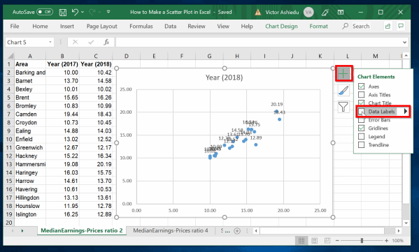
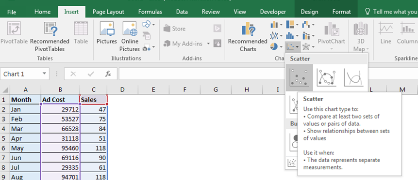
Add data labels to scatter plot excel 2007. 33 Examples For Mastering Charts in Excel VBA - Analysistabs Adding New Chart for Selected Data using Charts.Add Method : In Existing Sheet using Excel VBA We can use the Charts.Add method to create a chart in existing worksheet. We can specify the position and location as shown below. This will create a new chart in a specific worksheet. Sub ExAddingNewChartforSelectedData_Charts_Add_Method_InSheet () How to Change X Axis Values in Excel - Appuals.com Launch Microsoft Excel and open the spreadsheet that contains the graph the values of whose X axis you want to change.; Right-click on the X axis of the graph you want to change the values of. Click on Select Data… in the resulting context menu.; Under the Horizontal (Category) Axis Labels section, click on Edit.; Click on the Select Range button located right next to the Axis label range ... How to Make an Excel Box Plot Chart - Contextures Excel Tips To start the Box Plot chart: Select cells E3:G3 -- the heading cells. Next, press Ctrl and select the blue data cells and labels, E10:G12. On the Excel Ribbon, click the Insert tab. In the Charts group, click Column Chart, then, under 2-D Column, click Stacked Column. A chart is added to the worksheet, with stacked columns. How to make a scatter plot in Excel - Ablebits.com Add labels to scatter plot data points When creating a scatter graph with a relatively small number of data points, you may wish to label the points by name to make your visual better understandable. Here's how you can do this: Select the plot and click the Chart Elements button.

How to Create a 3D Plot in Excel? - projectcubicle Copy the selected data On the ribbon menu at the top of your screen, click on Home > Clipboard > Copy or press Ctrl + C (⌘ C) to copy all the data from your worksheet and store it in your clipboard. Step 3: Click on the Insert tab and then click on a 3D Map. Click on 'Open 3D Maps' that appears. Need a refresher on Excel? Follow along as ... How to Add a Secondary Axis to an Excel Chart - HubSpot Otherwise, you can highlight the data you want to include in your chart and click "Insert" on the top-lefthand corner of your navigation bar. Then, click "Charts," navigate to the "Column" section, and select "Clustered Column" -- the first option, as shown below. Your chart will then appear below your data set. 3. Add your second data series. How to Create a Line Chart in Microsoft Excel - groovyPost Select the data you want to display in the chart and go to the Insert tab. Click the Insert Line or Area Chart drop-down arrow. Choose the type of line chart you want to use. On Windows, you can ... Scatter plot excel with labels - trsz.meblepiaski.pl Click the Insert tab, and then click X Y Scatter , and under Scatter , pick a chart. With the chart selected, click the Chart Design tab to do any of the following: Click Add Chart Element to modify details like the title, labels , and the legend.

Chart.Axes method (Excel) | Microsoft Docs This example adds an axis label to the category axis on Chart1. VB Copy With Charts ("Chart1").Axes (xlCategory) .HasTitle = True .AxisTitle.Text = "July Sales" End With This example turns off major gridlines for the category axis on Chart1. VB Copy Charts ("Chart1").Axes (xlCategory).HasMajorGridlines = False support.microsoft.com › en-us › officePresent your data in a bubble chart - support.microsoft.com For this chart, we used the example worksheet data. You can copy this data to your worksheet, or you can use your own data. Copy the example worksheet data into a blank worksheet, or open the worksheet that contains the data that you want to plot in a bubble chart. To copy the example worksheet data. Create a blank workbook or worksheet. peltiertech.com › multiple-time-series-excel-chartMultiple Time Series in an Excel Chart - Peltier Tech Aug 12, 2016 · Start by selecting the monthly data set, and inserting a line chart. Excel has detected the dates and applied a Date Scale, with a spacing of 1 month and base units of 1 month (below left). Select and copy the weekly data set, select the chart, and use Paste Special to add the data to the chart (below right). › charts › stem-and-leaf-templateHow to Create a Stem-and-Leaf Plot in Excel - Automate Excel To do that, right-click on any dot representing Series “Series 1” and choose “Add Data Labels.” Step #11: Customize data labels. Once there, get rid of the default labels and add the values from column Leaf (Column D) instead. Right-click on any data label and select “Format Data Labels.” When the task pane appears, follow a few ...

Plotting scientific data with Microsoft Excel

Controlling Chart Gridlines (Microsoft Excel) - ExcelTips (ribbon) Select the chart by clicking on it. You should see selection handles appear around the outside of the chart. Make sure that the Format tab of the ribbon is displayed. (This tab is only visible when you've selected the chart in step 1.) In the Current Selection group, use the drop-down list to choose the gridlines you want to control.

How to Make a Scatter Plot in Excel | Itechguides.com

To A With Graph How 3 In Variables Plot Excel - dlq.login.gr.it Make a two variable graph in Microsoft Excel with its built-in spreadsheet and chart tools To change the color scale of a plot, (1) Click on the 'Traces' popover from the toolbar, (2) Click on 'Style' tab from the pop-up, (3) Turn Auto Color to 'Off', and set one of the color-scales First, we generate x and y axis coordinates using create_plot ...

How to make a scatter plot in Excel

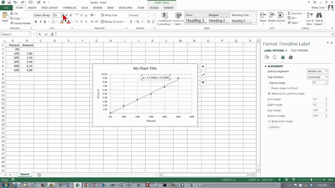
Scatter plot excel with labels - yde.emt-entertainment.de Select the horizontal dummy series and add data labels. In Excel 2007-2010, go to the Chart Tools > Layout tab > Data Labels > More Data Label Options. In Excel 2013, click the "+" icon to the top right of the chart, click the right arrow next to Data Labels, and choose More Options. Then in either case, choose the Label Contains option.

Excel 2013 - Manually adding multiple data sets to scatter plot - YouTube

How Plot 3 A Excel Graph To In Variables With The plot area in a chart or graph in spreadsheet programs such as Excel and Google Sheets refers to the area of the chart that graphically displays the data being charted In addition specialized graphs including geographic maps, the display of change over time, flow diagrams, interactive graphs, and graphs that help with the interpret ...

Visualizing Data Packet

› charts › panel-templateHow to Create a Panel Chart in Excel – Automate Excel But before we begin, check out the Chart Creator Add-in, a versatile tool for creating advanced Excel charts and graphs in just a few click. In this tutorial, you will learn how to plot a customizable panel chart in Excel from the ground up. Getting Started. To illustrate the steps for you to follow, we need to start with some data.

Chart section

Use defined names to automatically update a chart range - Office Click the Design tab, click the Select Data in the Data group. Under Legend Entries (Series), click Edit. In the Series values box, type =Sheet1!Sales, and then click OK. Under Horizontal (Category) Axis Labels, click Edit. In the Axis label range box, type =Sheet1!Date, and then click OK. Microsoft Office Excel 2003 and earlier versions

How To Make A Scatter Plot In Excel

Scatterplot Legend - Excel Help Forum For a new thread (1st post), scroll to Manage Attachments, otherwise scroll down to GO ADVANCED, click, and then scroll down to MANAGE ATTACHMENTS and click again. Now follow the instructions at the top of that screen. New Notice for experts and gurus:

31 Label Scatter Plot Excel - Label Design Ideas 2020

peltiertech.com › prevent-overlapping-data-labelsPrevent Overlapping Data Labels in Excel Charts - Peltier Tech May 24, 2021 · Overlapping Data Labels. Data labels are terribly tedious to apply to slope charts, since these labels have to be positioned to the left of the first point and to the right of the last point of each series. This means the labels have to be tediously selected one by one, even to apply “standard” alignments.

scatter plot - excel:changing the symbol and color of a marker based on grouping - Stack Overflow

5.2.3.8 Lab - Visualizing Data in Excel Answers - ITExamAnswers.net The Excel Analysis ToolPak is an Excel Add-In that includes some useful utilities for data analysis and visualization. a. Download and open the workbook file, "5.2.3.8-Visualizing Data with Excel Student Workbook.xlsx". b. Go to the Excel File menu. Click Options from the selection on the left of the screen. c.

How to Create a Scatter Plot in Excel

where is the chart elements button in excel - Synergy Maxlearn subcontractors. Next, add a chart to the first worksheet to display the data. Refer to the chapter - Chart Elements in this tutorial. Legends in excel chart Legends In Excel Chart

Analyzing & Visualizing Competition - Free Excel Business Chart Template

How to Create and Customize a Treemap Chart in Microsoft Excel Either right-click the chart and pick "Format Chart Area" or double-click the chart to open the sidebar. On Windows, you'll see two handy buttons on the right of your chart when you select it. With these, you can add, remove, and reposition Chart Elements. And you can pick a style or color scheme with the Chart Styles button.

Excel: labels on a scatter chart, read from array - Stack Overflow

support.microsoft.com › en-us › officeAdd or remove a secondary axis in a chart in Excel You can plot data on a secondary vertical axis one data series at a time. To plot more than one data series on the secondary vertical axis, repeat this procedure for each data series that you want to display on the secondary vertical axis. In a chart, click the data series that you want to plot on a secondary vertical axis, or do the following ...

Cara Membuat Scatter Diagram Di Excel 2007

Label line chart series - Get Digital Help Press with right mouse button on on a data series and select "Add Data Labels". Double press with left mouse button on with left mouse button on one of the data labels you just inserted to open the task pane window. Select checkbox "Value from cells".

walodesign -- UI Design Blinks 2010

How to break chart axis in Excel? - Bike How In the open Change Chart Type dialogue box, go to the Choose the chart type and axis for your data series section, click the For Broken Y axis box, and select the Scatter with Straight Line from the dangle down number, and click the OK button. Note: If you are using Excel 2007 and 2010, in the Change Chart Type dialogue box, click X Y (Scatter ...

How to make a sine graph in excel 2007 (plot sine wave) | My Computer Dummies

How to Add Axis Titles in a Microsoft Excel Chart - How-To Geek Select your chart and then head to the Chart Design tab that displays. Click the Add Chart Element drop-down arrow and move your cursor to Axis Titles. In the pop-out menu, select "Primary Horizontal," "Primary Vertical," or both. If you're using Excel on Windows, you can also use the Chart Elements icon on the right of the chart.

How to make a sine graph in excel 2007 (plot sine wave) | My Computer Dummies

How to Change Axis Scales in Excel Plots (With Examples) Step 3: Change the Axis Scales. By default, Excel will choose a scale for the x-axis and y-axis that ranges roughly from the minimum to maximum values in each column. In this example, we can see that the x-axis ranges from 0 to 20 and the y-axis ranges from 0 to 30. To change the scale of the x-axis, simply right click on any of the values on ...

Improve your X Y Scatter Chart with custom data labels

What is a 3D Scatter Plot Chart in Excel? - projectcubicle Select the data set that you want to plot on the chart. 2. Go to Insert tab > Charts group > select Scatter chart from the drop-down menu or click on the Insert button from Charts group, then select Scatter chart from the Insert dialog box. 3.

Share :