43 change data labels in excel chart

How to change chart axis labels' font color and size in Excel? Apply conditional formatting to fill columns in a chart. By default, all data point in one data series are filled with same color. Here, with the Color Chart by Value tool of Kutools for Excel, you can easily apply conditional formatting to a chart, and fill data points with different colors based on point values. Full Feature Free Trial 30-day! › how-to-create-excel-pie-chartsHow to Make a Pie Chart in Excel & Add Rich Data Labels to ... Sep 08, 2022 · In this article, we are going to see a detailed description of how to make a pie chart in excel. One can easily create a pie chart and add rich data labels, to one’s pie chart in Excel. So, let’s see how to effectively use a pie chart and add rich data labels to your chart, in order to present data, using a simple tennis related example.

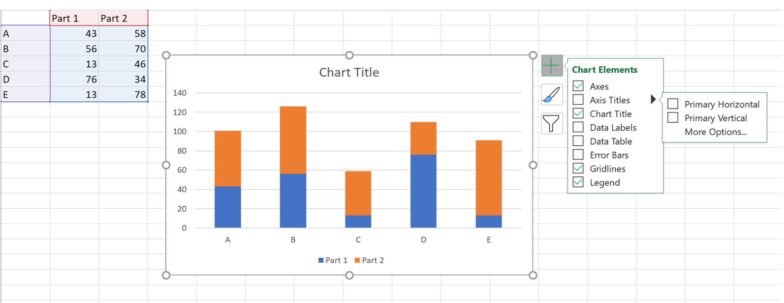
Add / Move Data Labels in Charts - Excel & Google Sheets Adding Data Labels Click on the graph Select + Sign in the top right of the graph Check Data Labels Change Position of Data Labels Click on the arrow next to Data Labels to change the position of where the labels are in relation to the bar chart Final Graph with Data Labels

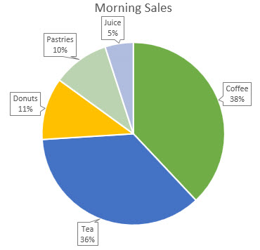
Change data labels in excel chart

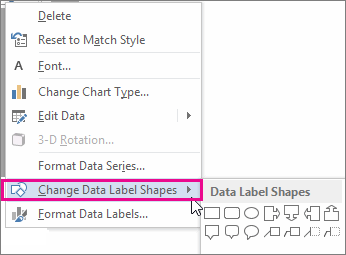
How to create Custom Data Labels in Excel Charts - Efficiency 365 Right click on any data label and choose the callout shape from Change Data Label Shapes option. Now adjust each data label as required to avoid overlap. Put solid fill color in the labels Finally, click on the chart (to deselect the currently selected label) and then click on a data label again (to select all data labels). How to add or move data labels in Excel chart? - ExtendOffice In Excel 2013 or 2016. 1. Click the chart to show the Chart Elements button . 2. Then click the Chart Elements, and check Data Labels, then you can click the arrow to choose an option about the data labels in the sub menu. See screenshot: In Excel 2010 or 2007. 1. click on the chart to show the Layout tab in the Chart Tools group. See ... Axis Chart Update Vba [YFCBR4] - 11.casaviva.genova.it The six labels show correctly in the select data preview screen, but not on the chart (just shows numbers 1 - 6) ) Excel displays the Format Axis dialog box An array of category values (January, February, and so forth) Here I have a excel table that consists sales data of employees Insert a 'Stacked Bar Chart' from the Insert menu Kohler ...

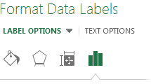
Change data labels in excel chart. Move data labels - support.microsoft.com Click any data label once to select all of them, or double-click a specific data label you want to move. Right-click the selection > Chart Elements > Data Labels arrow, and select the placement option you want. Different options are available for different chart types. support.microsoft.com › en-us › officeChange the format of data labels in a chart To get there, after adding your data labels, select the data label to format, and then click Chart Elements > Data Labels > More Options. To go to the appropriate area, click one of the four icons ( Fill & Line , Effects , Size & Properties ( Layout & Properties in Outlook or Word), or Label Options ) shown here. excel - How do I update the data label of a chart? - Stack Overflow To build your data labels, somewhere else on your worksheet (conveniently, in the adjacent column would be ideal), use Excel formula to build the desired label string, for example: ="Blue occupies "&TEXT(B3,"0%") Repeat for the other points in the chart. Once you've done that, here's how you link Data Labels to a cell reference (normally, Data ... How to Use Cell Values for Excel Chart Labels - How-To Geek Select the chart, choose the "Chart Elements" option, click the "Data Labels" arrow, and then "More Options." Uncheck the "Value" box and check the "Value From Cells" box. Select cells C2:C6 to use for the data label range and then click the "OK" button. The values from these cells are now used for the chart data labels.

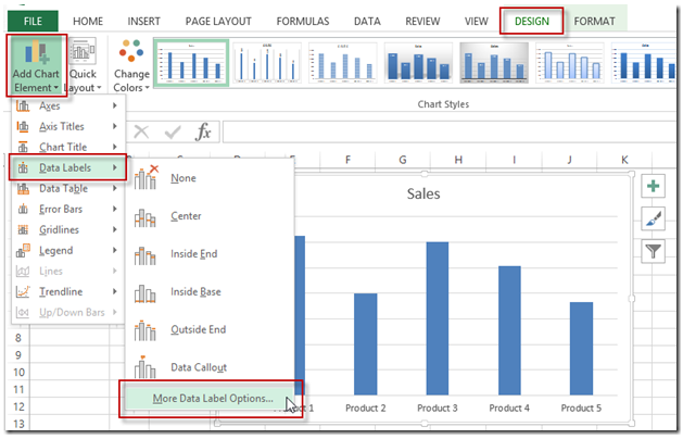
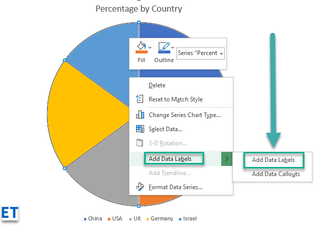
Add or remove data labels in a chart - support.microsoft.com Click the data series or chart. To label one data point, after clicking the series, click that data point. In the upper right corner, next to the chart, click Add Chart Element > Data Labels. To change the location, click the arrow, and choose an option. If you want to show your data label inside a text bubble shape, click Data Callout. How do I replicate an Excel chart but change the data? 18.10.2018 · If you have created a Mekko Graphics chart in Excel, you can use the same chart again, but with different data. Here's an example of how to re-use a cascade/waterfall chart . Select the Excel chart (single click) and then right click to choose Copy. › excel › how-to-add-total-dataHow to Add Total Data Labels to the Excel Stacked Bar Chart Apr 03, 2013 · Step 4: Right click your new line chart and select “Add Data Labels” Step 5: Right click your new data labels and format them so that their label position is “Above”; also make the labels bold and increase the font size. Step 6: Right click the line, select “Format Data Series”; in the Line Color menu, select “No line” How to Customize Your Excel Pivot Chart Data Labels - dummies The Data Labels command on the Design tab's Add Chart Element menu in Excel allows you to label data markers with values from your pivot table. When you click the command button, Excel displays a menu with commands corresponding to locations for the data labels: None, Center, Left, Right, Above, and Below. None signifies that no data labels ...

Question: labels in an Excel doughnut chart Open your Excel document and click on your chart. In the upper bar you will find the "Diagram Tools". Click on the "Design" tab. In the "Data" group, click the "Select Data" button. In the left window you will find the legend entries. Click on an entry and select "Edit". You can now rename the entry under "Row name". How to make a histogram in Excel 2019, 2016, 2013 and 2010 Make a histogram using Excel's Analysis ToolPak. With the Analysis ToolPak enabled and bins specified, perform the following steps to create a histogram in your Excel sheet: On the Data tab, in the Analysis group, click the Data Analysis button. In the Data Analysis dialog, select Histogram and click OK. In the Histogram dialog window, do the ... How to Make a Pie Chart in Excel & Add Rich Data Labels to The Chart! 08.09.2022 · A pie chart is used to showcase parts of a whole or the proportions of a whole. There should be about five pieces in a pie chart if there are too many slices, then it’s best to use another type of chart or a pie of pie chart in order to showcase the data better. In this article, we are going to see a detailed description of how to make a pie chart in excel. Edit titles or data labels in a chart - support.microsoft.com Change the position of data labels. You can change the position of a single data label by dragging it. You can also place data labels in a standard position relative to their data markers. Depending on the chart type, you can choose from a variety of positioning options. On a chart, do one of the following:

Add or remove data labels in a chart

How to add data labels from different column in an Excel chart? Right click the data series in the chart, and select Add Data Labels > Add Data Labels from the context menu to add data labels. 2. Click any data label to select all data labels, and then click the specified data label to select it only in the chart. 3.

Change Horizontal Axis Values in Excel 2016 - AbsentData

How to Change Excel Chart Data Labels to Custom Values? 05.05.2010 · Now, click on any data label. This will select “all” data labels. Now click once again. At this point excel will select only one data label. Go to Formula bar, press = and point to the cell where the data label for that chart data point is defined. Repeat the process for all other data labels, one after another. See the screencast.

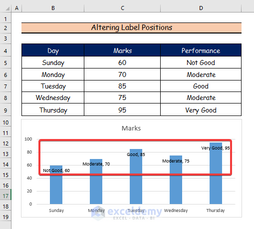
How to Edit Data Labels in Excel (6 Easy Ways) - ExcelDemy

chandoo.org › wp › change-data-labels-in-chartsHow to Change Excel Chart Data Labels to Custom Values? May 05, 2010 · Now, click on any data label. This will select “all” data labels. Now click once again. At this point excel will select only one data label. Go to Formula bar, press = and point to the cell where the data label for that chart data point is defined. Repeat the process for all other data labels, one after another. See the screencast.

excel - VBA Change Data Labels on a Stacked Column chart from ...

How to Add Data Labels to an Excel 2010 Chart - dummies On the Chart Tools Layout tab, click Data Labels→More Data Label Options. The Format Data Labels dialog box appears. You can use the options on the Label Options, Number, Fill, Border Color, Border Styles, Shadow, Glow and Soft Edges, 3-D Format, and Alignment tabs to customize the appearance and position of the data labels.

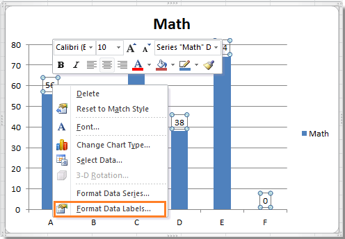
How to hide zero data labels in chart in Excel?

support.microsoft.com › en-us › officeEdit titles or data labels in a chart - support.microsoft.com Change the position of data labels. You can change the position of a single data label by dragging it. You can also place data labels in a standard position relative to their data markers. Depending on the chart type, you can choose from a variety of positioning options. On a chart, do one of the following:

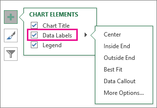
Add or remove data labels in a chart

Dynamically Label Excel Chart Series Lines - My Online Training … 26.09.2017 · Hi Mynda – thanks for all your columns. You can use the Quick Layout function in Excel (Design tab of the chart) to do the labels to the right of the lines in the chart. Use Quick Layout 6. You may need to swap the columns and rows in your data for it to show. Then you simply modify the labels to show only the series name. I just happened to ...

Custom Data Labels with Colors and Symbols in Excel Charts ...

Change axis labels in a chart - support.microsoft.com Right-click the category labels you want to change, and click Select Data. In the Horizontal (Category) Axis Labels box, click Edit. In the Axis label range box, enter the labels you want to use, separated by commas. For example, type Quarter 1,Quarter 2,Quarter 3,Quarter 4. Change the format of text and numbers in labels

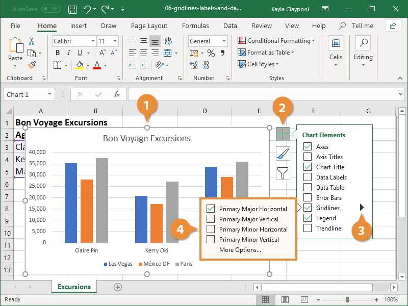
How to Add Axis Labels to a Chart in Excel | CustomGuide

Is there a way to change the order of Data Labels? Answer Rena Yu MSFT Microsoft Agent | Moderator Replied on April 4, 2018 Hi Keith, I got your meaning. Please try to double click the the part of the label value, and choose the one you want to show to change the order. Thanks, Rena ----------------------- * Beware of scammers posting fake support numbers here.

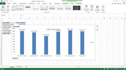
How to Customize Your Excel Pivot Chart Data Labels - dummies

How to Change Chart Data Range in Excel (5 Quick Methods) - ExcelDemy 1. Using Design Tab to Change Chart Data Range in Excel. There is a built-in process in Excel for making charts under the Charts group Feature.In addition, I need a chart to see you how to change that chart data range.Here, I will use Bar Charts Feature to make a Bar Chart.The steps are given below.

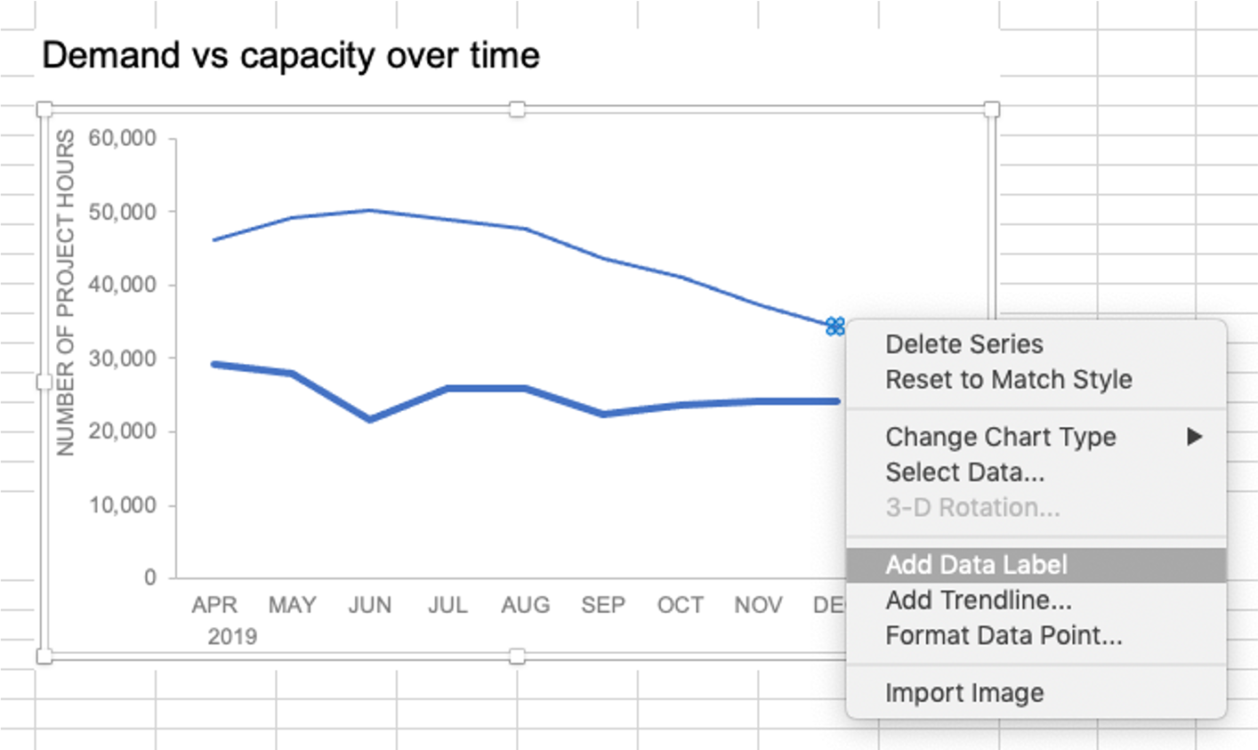
how to add data labels into Excel graphs — storytelling with data

How to Add Data Labels in Excel - Excelchat | Excelchat In Excel 2013 and the later versions we need to do the followings; Click anywhere in the chart area to display the Chart Elements button Figure 5. Chart Elements Button Click the Chart Elements button > Select the Data Labels, then click the Arrow to choose the data labels position. Figure 6. How to Add Data Labels in Excel 2013 Figure 7.

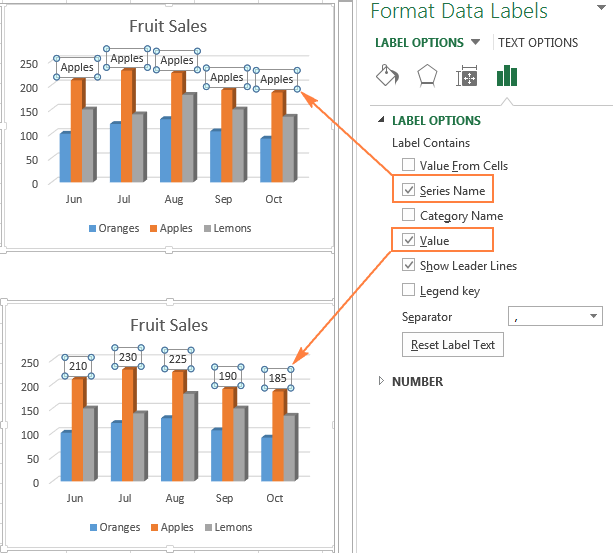
Excel charts: add title, customize chart axis, legend and ...

› how-do-i-replicate-anHow do I replicate an Excel chart but change the data? Oct 18, 2018 · To update the data range, double click on the chart, and choose Change Date Range from the Mekko Graphics ribbon. Select your new data range and click OK in the floating Chart Data dialog box. Your data can be in the same worksheet as the chart, as shown in the example below, or in a different worksheet.

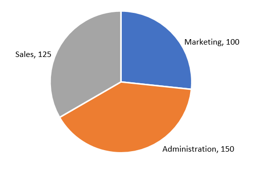
How to fix wrapped data labels in a pie chart | Sage Intelligence

How to rotate axis labels in chart in Excel? - ExtendOffice Rotate axis labels in Excel 2007/2010. 1. Right click at the axis you want to rotate its labels, select Format Axis from the context menu. See screenshot: 2. In the Format Axis dialog, click Alignment tab and go to the Text Layout section to select the direction you need from the list box of Text direction. See screenshot: 3. Close the dialog ...

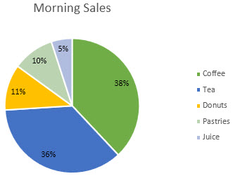
Change the format of data labels in a chart

How to Edit Pie Chart in Excel (All Possible Modifications) How to Edit Pie Chart in Excel 1. Change Chart Color 2. Change Background Color 3. Change Font of Pie Chart 4. Change Chart Border 5. Resize Pie Chart 6. Change Chart Title Position 7. Change Data Labels Position 8. Show Percentage on Data Labels 9. Change Pie Chart's Legend Position 10. Edit Pie Chart Using Switch Row/Column Button 11.

Adding rich data labels to charts in Excel 2013 | Microsoft ...

Custom Data Labels with Colors and Symbols in Excel Charts - [How To ... Step 4: Select the data in column C and hit Ctrl+1 to invoke format cell dialogue box. From left click custom and have your cursor in the type field and follow these steps: Press and Hold ALT key on the keyboard and on the Numpad hit 3 and 0 keys. Let go the ALT key and you will see that upward arrow is inserted.

Format Data Labels in Excel- Instructions - TeachUcomp, Inc.

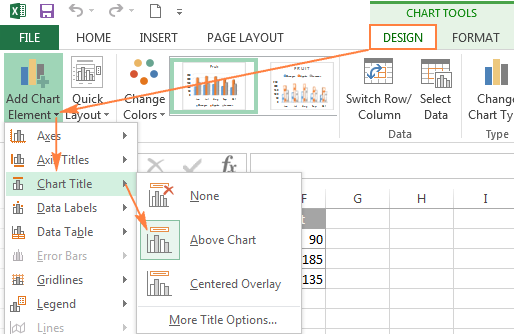
Adding Data Labels to Your Chart (Microsoft Excel) - ExcelTips (ribbon) Select the position that best fits where you want your labels to appear. To add data labels in Excel 2013 or later versions, follow these steps: Activate the chart by clicking on it, if necessary. Make sure the Design tab of the ribbon is displayed. (This will appear when the chart is selected.) Click the Add Chart Element drop-down list.

Google Workspace Updates: Get more control over chart data ...

Data Labels in Excel Pivot Chart (Detailed Analysis) Next open Format Data Labels by pressing the More options in the Data Labels. Then on the side panel, click on the Value From Cells. Next, in the dialog box, Select D5:D11, and click OK. Right after clicking OK, you will notice that there are percentage signs showing on top of the columns. 4. Changing Appearance of Pivot Chart Labels

Change color of data label placed, using the 'best fit ...

Modify Excel Chart Data Range | CustomGuide Once you see data in a chart, you may find there are some tweaks and changes that need to be made. Here are a few ways to change the data in your chart. Add a Data Series. If you need to add additional data from the spreadsheet to the chart after it’s created, you can adjust the source data area. Select the chart.

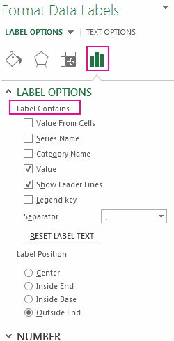
Add or remove data labels in a chart

Create Dynamic Chart Data Labels with Slicers - Excel Campus Bottom line: Learn how to create this interactive chart where the data label metrics change based on a slicer. Skill level: Advanced. ... Typically a chart will display data labels based on the underlying source data for the chart. In Excel 2013 a new feature called "Value from Cells" was introduced. This feature allows us to specify the a ...

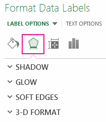
Change the format of data labels in a chart

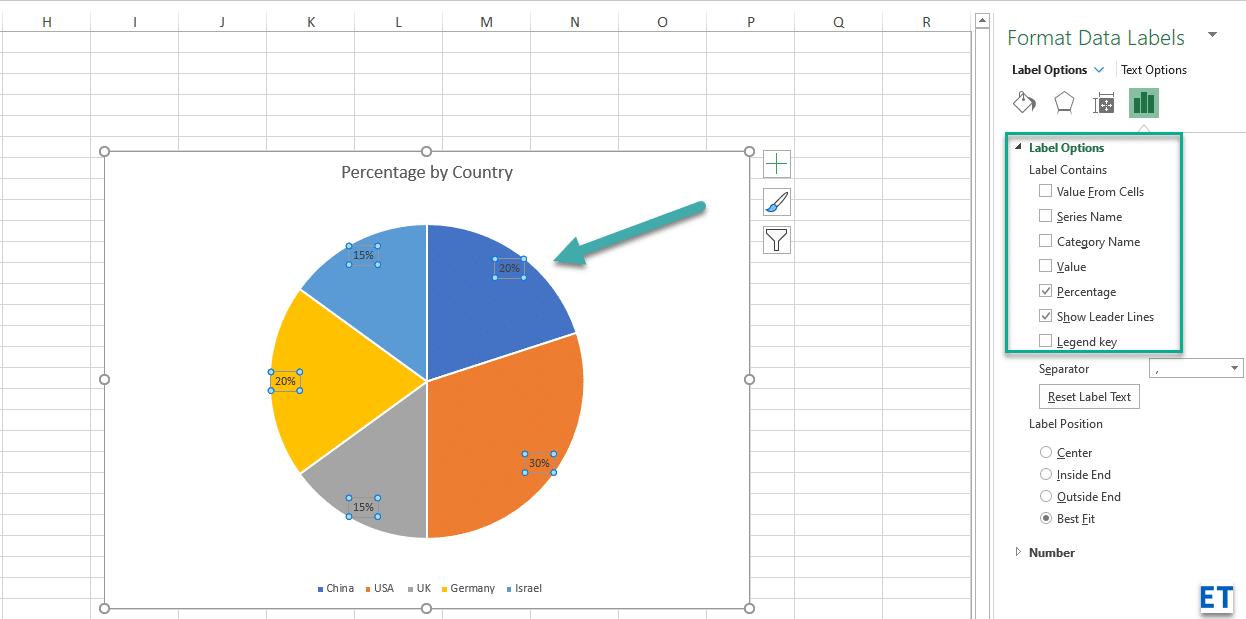
Change the format of data labels in a chart To get there, after adding your data labels, select the data label to format, and then click Chart Elements > Data Labels > More Options. To go to the appropriate area, click one of the four icons ( Fill & Line , Effects , Size & Properties ( Layout & Properties in Outlook or Word), or Label Options ) shown here.

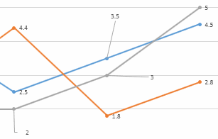
Change the format of data labels in a chart

2/ Right-click i.e. on the 1st histo. bar (A) > Add Data Labels (numbers are displayed a the top of the bars) 3/ Click one of the numbers that just displayed (the Format Data Labels pane opens on the right) > Check option "Value From Cells" > Select range C2:C7 > OK > Uncheck option "Value" demo.png(18.5 KiB) Comment Comment ·

Color Negative Chart Data Labels in Red with downward arrow

How to Add Total Data Labels to the Excel Stacked Bar Chart 03.04.2013 · Step 2: Right click the new data series and select “Change series Chart Type…” Step 3: Choose one of the simple line charts as your new Chart Type. Step 4: Right click your new line chart and select “Add Data Labels” Step 5: Right click your new data labels and format them so that their label position is “Above”; also make the labels bold and increase the font …

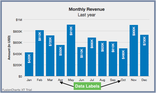
Display Customized Data Labels on Charts & Graphs

› documents › excelHow to change chart axis labels' font color and size in Excel? Sometimes, you may want to change labels' font color by positive/negative/0 in an axis in chart. You can get it done with conditional formatting easily as follows: 1. Right click the axis you will change labels by positive/negative/0, and select the Format Axis from right-clicking menu. 2. Do one of below processes based on your Microsoft Excel ...

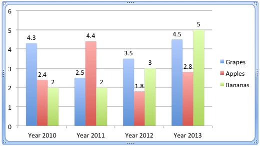
Format Number Options for Chart Data Labels in Excel 2011 for Mac

Custom Chart Data Labels In Excel With Formulas Follow the steps below to create the custom data labels. Select the chart label you want to change. In the formula-bar hit = (equals), select the cell reference containing your chart label's data. In this case, the first label is in cell E2. Finally, repeat for all your chart laebls.

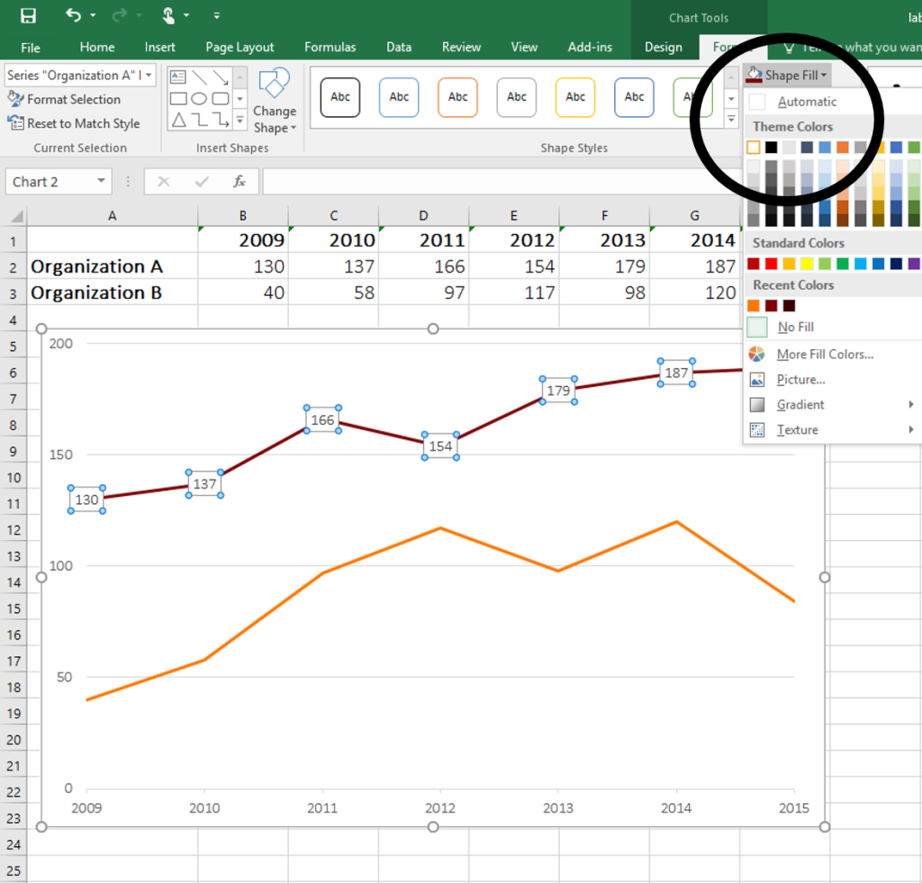
How to Place Labels Directly Through Your Line Graph in ...

Axis Chart Update Vba [YFCBR4] - 11.casaviva.genova.it The six labels show correctly in the select data preview screen, but not on the chart (just shows numbers 1 - 6) ) Excel displays the Format Axis dialog box An array of category values (January, February, and so forth) Here I have a excel table that consists sales data of employees Insert a 'Stacked Bar Chart' from the Insert menu Kohler ...

Enable or Disable Excel Data Labels at the click of a button ...

How to add or move data labels in Excel chart? - ExtendOffice In Excel 2013 or 2016. 1. Click the chart to show the Chart Elements button . 2. Then click the Chart Elements, and check Data Labels, then you can click the arrow to choose an option about the data labels in the sub menu. See screenshot: In Excel 2010 or 2007. 1. click on the chart to show the Layout tab in the Chart Tools group. See ...